Quick Tutorial¶

Installation/Usage¶

As the package has not been published on PyPi yet, it CANNOT be install using pip.

For now, the suggested method is to put the file Complex_Contagions.py in the same directory as your source files and call from Complex_Contagions import geometric_network

Initiate a `geometric_network` object¶

Create a geometric network on a ring. Band_length corresponds to the number of neighbors to connect from both right and left making the geometric degree 2*band_length

n = 20
d2 = 2
ring_latt=  geometric_network('ring_lattice', size = n, banded = True, band_length = 3)

Add noise to geometric network¶

Use add_noise_to_geometric() method to manipulate the network topology. The second parameter describes the non-geometric degree of every node.

ring_latt_k_regular.add_noise_to_geometric('k_regular', d2)

Display the network via Networkx¶

Spy the network.

ring_latt_k_regular.display()

Sample Excitation Simulation¶

Run the complex contagion on the network we have created. Key parameters are threshold, C and $alpha = frac{nGD}{GD}$

n = 200
d2 = 2
ring_latt_k_regular =  geometric_network('ring_lattice', size = n, banded = True, band_length = 3)
ring_latt_k_regular.add_noise_to_geometric('k_regular', d2)

T = 100 # number of iterations
seed = int(n/2) # node that the spread starts
C = 1000 # Geometrically, this describes the turning of the sigmoid function
threshold = 0.3 # resistence of the node to it's neighbors' excitation level
Trials = 2 # number of trials
refractory_period = False ## if a neuron is activated once, it stays activated throughout.

fig, ax = plt.subplots(Trials,1, figsize = (50,10))
first_excitation_times, contagion_size = ring_latt_k_regular.run_excitation(Trials, T, C, seed, threshold, refractory_period, ax = ax)

The way excitation spreads along time. Since we have chosen a high value of C, the model tends to be more deterministic which explains the highly similar behavoir between different Trials.

Look at the first activation times¶

Spy activation of the nodes.

ring_latt_k_regular.spy_first_activation(first_excitation_times)

As we mentioned, the activation times are exactly the same in both trials since the model is deterministic.

Create Distance Matrix¶

If you don’t need to look at the individual contagions starting from different nodes, you can run the contagion starting from node i and calculating the first time it reaches to node j i.e. create a distance matrix who (i,j) entry is the first time the node j activated on a contagion starting from i.

D, Q = ring_latt_k_regular.make_distance_matrix(T, C, threshold, Trials, refractory_period, spy_distance = True)

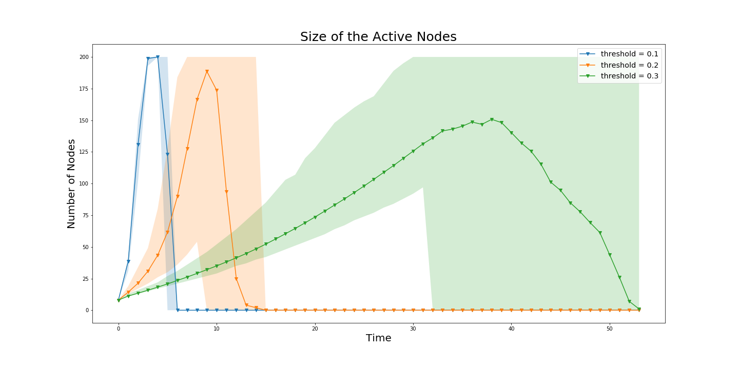
Contagion Size¶

It’s important to look at the bifurcations in the system. In order to do so, one might need to look at the size of the contagion for example different thresholds.

labels = ['threshold = 0.1', 'threshold = 0.2', 'threshold = 0.3']
Q = [Q1,Q2,Q3]  ## Qi is the second output of the ``make_distance_matrix``
ring_latt_k_regular.display_comm_sizes(Q,labels)

The sizes of the contagion for different thresholds. Shade indicates the max and min values of the contagion starting from different nodes.

Persistence Diagrams¶

Once we created the distance matrices, we can look at the topological features across different contagions and different topologies.

pers = ring_latt_k_regular.compute_persistence(D, spy = True)
delta = ring_latt_k_regular.one_d_Delta(pers)

Persistence diagram computed from the distance matrix via Rips filtration. Green is 1-D features, red is 0-D features.